Create Dynamic Range for your Charts

Hi guys recently I got an email where the sender has requested to create chart in such a manner that graph adjusts itself to the changing figures in the table or data. I provide him a solution which look something like the below image.
Download the file from here: DYNAMIC RANGE

Now the real question here comes is, how this was done? For that I have used Name Manager from Formulas tab.  Don't worry I will tell you step by step process to create this chart and dynamic data input range for it.

Suppose I have a table like given in the image below and I want to create a chart for this table in such way that if I enter Budget and Actual sales in column C & D, these values will automatically get reflected in my chart.
Now first I will name my ranges to be plotted in charts. For that click Formulas > Name Manager > New

For Budget column name it as Budget_data or whatever you like and in refers to box at the bottom write the formula as =OFFSET(Sheet1!$C$5,0,0,COUNT(Sheet1!$C$5:$C$16)). Similarly for 2011 data name it as Actual_data and refers to =OFFSET(Sheet1!$D$5,0,0,COUNT(Sheet1!$D$5:$D$16))  have a look at the image below.
Before moving ahead I want to explain what the above formula is doing.  To put it in layman language, OFFSET is helping us to select the range starting from C5 and COUNT function is helping the formula to decide the height of range by counting the number of data entered in the table.

Once we're done naming ranges now we'll create charts and do edits required to make it dynamic.
Select your data to be plotted, here select B4:D15 and click Insert > Charts > Column > Clustered Column.  It will give you a chart appearing as in 1 of image below.

Now right click in your chart and select change series chart type as in 2 of the image.  Select Line chart type.

You can also change the layout of your chart and tittle as done in 3 of the image.

Now in 4 comes the most important part of this trick.  Here we will adjust the data source for our chart and define the two series shown in the chart.
As shown in 4 of the above image, when we click Select Data it will open Select Data Source Box where under Legend Entries (Series) we'll edit Series1 & Series2.  In the following image below we have made edits to Series1 by referring Series name to cell C3 & Series values to "Budget_Data" which we named above.  Similarly for Series2 we referred Series name to cell D3 & Series values to "Actual_Data".
What this will do is make our chart responsive to the data we enter in table range B4:D15.  When we enter figures for any month it will automatically plot the same in the corresponding chart.  And that exactly was our goal as well.

Hope you learned something out of this trick.  "HAPPY LEARNING"

Conditional Lookup using Multi Criteria

Hello readers today's post will be short but I assure you it will help you tackle problem which you may be facing or might face in future. Suppose you want to look up any value based on two criteria, for example in the below image you want to know the price in F8 based on Make & Color in F2 & F5 respectively.
I know the solution to this can be found using filter feature, but being big fan of functions I would like to provide you formula to find it as well.  You'll use a combination of INDEX & MATCH function to get your figure here. The formula in F8 will be as follows:
F8: {=INDEX(C2:C10,MATCH(F2&F5,A2:A10&B2:B10,0))}
This is an array formula and to make it works you'll have to press (Ctrl+Shift+Enter) CSE.

Download sample file: MULTI-CRITERIA LOOKUP

Are you above or below AVERAGE in Excel?

AVERAGE this word is no new to any of us and it's meaning is known to all of us.  But what does it exactly means? The literal meaning is "a quantity, rating, or the like that represents or approximates an arithmetic mean".  For statistician it has always meant Arithmetic Mean and when used as an adjective it means typical; common; or ordinary. For example "Prakash has AVERAGE excel skills".

Today I am trying to throw some light on AVERAGE function in excel but will also talk about AVERAGEA, AVERAGEIF & AVERAGEIFS.  So be with this post and by the time you finish reading, you'll be equipped with the power of four functions of excel in a matter of few minutes.

AVERAGE function as described in Excel Help is "Returns the average (arithmetic mean) of the arguments." For example, if the range A1:M1 contains numbers, the formula =AVERAGE(A1:M1) returns the average of those numbers.  See the image below explaining this situation:
Things one should know about AVERAGE function are provided arguments can either be numbers or names, ranges, or cell cell references that contains numbers.  Also if a range or cell reference contains text, logical values, or empty cells, those values are ignored; however, cells with negative or zero value are included for calculation of average.

Now what should one do if his data also has negative or zero values and he is looking to get average of only positive values.  Got stuck? Don't worry there is always a solution for every problem, and this riddle can also be solved.  You just need to know the way to approach it.  The formula created by using combination of SUMIF & COUNTIF as =SUMIF(A1:M1,">0")/COUNTIF(A1:M1,">0") can provide us a solution. If you've any other way to solve our problem, please share with our readers in comments at the end of the post.
Now I believe you guys know the AVERAGE function and are ready to go ahead and study other related fuctions I mentioned in the beginning.  First to go is AVERAGEA, this function also provides arithmetic mean but it doesn't ignore logical values and text in arguments.  Empty cell in the range is still ignored by this function as well.  For example in the below you see AVERAGEA(A1:M1) & AVERAGEA(A1:M1,N1) is giving us same result because blank cell N1 is ignored for calculation by function AVERAGEA.
It may also be possible that during your course of routine you would like to know or find average based on single or multiple criteria.  For example you want to calculate the average for numbers above 30 or average for values belonging to a particular category and are above 30 as well.  For situations like these excel has two powerful functions known as AVERAGEIF & AVERAGEIFS for single and multi criteria respectively.
In the image above AVERAGEIF function has been used to calculate average in the range A1:M2 provide that the values are greater than 30. At the same time AVERAGEIFS is being used to satisfy two conditions and calculate average.  Two conditions here are the number should belong to A2 category and should be greater than 30 as well.

So this way today you've added or refreshed functions related to averages in your knowledge base. Let me know about your past or present experiences of using these amazing functions in comments.  "HAPPY LEARNING"

Sum Using Multiple Criteria - SUMPRODUCT

SUMPRODUCT Function is used to sum a range when multiple conditions are met..

The first argument of sumproduct is the range which is to be summed.

Suppose you want to get a sum of a product range which falls between two Dates, In other words, the value in the amount range is summed only if both of the following criteria are met:

First condition: The Product should be Samsung..
Second condition: The range of the Date should be between 1-Jan-2001 & 22-Jan-2001

Here in this example my data is in Range A1:C38 & the conditions to be met are in E1:F3.
The below image is an extract from the worksheet.
The formula I have derived to get the solution is as follows:
=SUMPRODUCT((A2:A38>=F1)*(A2:A38<=F2)*(B2:B38=F3),C2:C38)

Put this formula and you will get the answer. This worksheet demonstrates summing based on multiple criteria. Download Sample File

This is a short and easy tip for time being, see you soon again.  "HAPPY LEARNING"


Insert a Blank Row after each Record without VBA

Hello friends I am back again with a new excel trick for you to learn.  Today I am trying to explain a very simple way to add a blank row after each record in your data.  This trick is very special because without VBA it is the only method to insert a blank row to your data except doing it manually.

Let me first tell you a little bit about the objective that I am planning to achieve. See the image below:
I want to insert a blank row after each record in my data. So there should be blank row between "Chris Smalling" & "Fabio" similarly between "Jonny" & "Nemanja". Now the challenge is to do it without using VBA codes. So here you go with the solution.

Enter a series of numbers in the column next to your data.  You can also use "Fill Handle" to put the series of numbers if your data is large, this is an efficient way of putting numbers.
Once you have numbers next to your data select the series and copy it. Go to the last number in the series and below it paste the full series again.
Now select your complete data along with the series entered. Here the series has been entered in column 2 and now sort it in ascending order with the column containing your number series.
Now if you see your original data has got a blank row after each record. This is what we were trying to achieve with this trick.  I know this can be done with a very simple VBA code, for my super efficient VBA loving friends I am posting the code in comments below.

I hope we you all have gained something out of this post. Your suggestions and feedback are most welcome. Till then "HAPPY LEARNING"

Dynamic Charts with Index & Match Function

Have you ever created a dynamic chart in excel? If yes, Kudos to you!  If not don't worry today you can master that skill in couple of minutes.  I would like to tell you that this is my first post on charts and I am starting a series on charting with this.  I will keep adding more to it time and again for sure.  In this post I'll be talking about how to create dynamic column chart using few amazing but simple functions of excel.  INDEX, MATCH & VALIDATION are three things I am using to create a dynamic chart which will look like the below example.


You can download the example from here! DYNAMIC CHART FILE

I am assuming that you have already downloaded the file from above.  In it you can see my main data is in range A1:E7, but using nested INDEX & MATCH functions I have created a new data for my chart to take in range A10:B16.

The challenge here is to change the data in range A10:B16.  If you see, you will notice that in cell H1 I have used data validation and it is giving me year for which I want my chart to plot the data. The data range A10:A16 has the name of car manufactures.  Using these two inputs I am pulling out data from main data.  The combination of functions I have used is as follows:

B11=INDEX($B$2:$E$7,MATCH($A11,$A$2:$A$7,0),MATCH($H$1,$B$1:$E$1,0))

Now I have dragged this function till B16 and I have my dynamic data ready with me.  It changes as I change the year in Cell H1.  Using this data series I have now created a chart.  To do it the steps are as follows:

Select your data > Insert > Charts > Column > 2-D Column > Clustered Column

You can now make adjustments as per your presentation requirement and give it a look as you want.  I have removed data labels from this chart and changed the color of each bar as well.  Just keep one thing in mind if you have the nested function mentioned above, rest of the work is simple.  You can use these charts in sales dashboards and many other places.  I use them it to show the performance of my team on weekly basis.

Dear reader, please let me know any feedback you have for me.  You can also give suggestions and topics that you want me to cover in upcoming posts.  Till then "HAPPY LEARNING!"

Sort Data from Left to Right (Sort data in Rows)

Dear readers & followers it's been a long time since my last post.  Now I have finally got some time to write something interesting and worth sharing. Today you're gonna learn how to sort data in rows. What I mean by that is sorting your data from left to right instead of sorting from top to bottom in column.

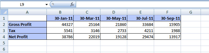
If you look at the image below it has few dates mentioned in column B to F and few figures for gross profit, tax & net profit associated with these dates.  Now what I am going to do is to sort these figures on the basis of dates in ascending order.
To do this what you'll have to do is follow a simple procedure and it will take very little time.  First of all select the data you want to sort and go to Home tab. There you'll find Sort & Filter option under Editing group.  Then you've to click on Custom Sort as shown in image below.
This will open a pop up box, at the top of it click on the Option button which will option Sort Options... box there look for Orientation and select Sort left to right.  By default it is Sort top to bottom.  This is shown in the image below.
Click OK and now you can see the option of sorting your data with rows.  Look at the sort by drop down option and you'll see Row1, Row2 etc now. Earlier it used to be Column1, Column2 and so on.
I've selected Row1, as my dates are in row 1 and I want to sort on their basis.  You can choose as per your requirement.  Oldest to Newest option under Order drop down will help us arrange the dates in required manner.  Click OK and here is what we intended to achieve.
Guys its easy and can be really helpful when you've to deal with large number of columns.  Hope you'll like my post, you can share your feedback or suggestion or any query via comments below. "HAPPY LEARNING"