Dynamic Charts with Index & Match Function

Have you ever created a dynamic chart in excel? If yes, Kudos to you!  If not don't worry today you can master that skill in couple of minutes.  I would like to tell you that this is my first post on charts and I am starting a series on charting with this.  I will keep adding more to it time and again for sure.  In this post I'll be talking about how to create dynamic column chart using few amazing but simple functions of excel.  INDEX, MATCH & VALIDATION are three things I am using to create a dynamic chart which will look like the below example.

You can download the example from here! DYNAMIC CHART FILE

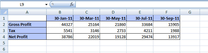
I am assuming that you have already downloaded the file from above.  In it you can see my main data is in range A1:E7, but using nested INDEX & MATCH functions I have created a new data for my chart to take in range A10:B16.

The challenge here is to change the data in range A10:B16.  If you see, you will notice that in cell H1 I have used data validation and it is giving me year for which I want my chart to plot the data. The data range A10:A16 has the name of car manufactures.  Using these two inputs I am pulling out data from main data.  The combination of functions I have used is as follows:

B11=INDEX($B$2:$E$7,MATCH($A11,$A$2:$A$7,0),MATCH($H$1,$B$1:$E$1,0))

Now I have dragged this function till B16 and I have my dynamic data ready with me.  It changes as I change the year in Cell H1.  Using this data series I have now created a chart.  To do it the steps are as follows:

Select your data > Insert > Charts > Column > 2-D Column > Clustered Column

You can now make adjustments as per your presentation requirement and give it a look as you want.  I have removed data labels from this chart and changed the color of each bar as well.  Just keep one thing in mind if you have the nested function mentioned above, rest of the work is simple.  You can use these charts in sales dashboards and many other places.  I use them it to show the performance of my team on weekly basis.

Dear reader, please let me know any feedback you have for me.  You can also give suggestions and topics that you want me to cover in upcoming posts.  Till then "HAPPY LEARNING!"

Sort Data from Left to Right (Sort data in Rows)

Dear readers & followers it's been a long time since my last post.  Now I have finally got some time to write something interesting and worth sharing. Today you're gonna learn how to sort data in rows. What I mean by that is sorting your data from left to right instead of sorting from top to bottom in column.

If you look at the image below it has few dates mentioned in column B to F and few figures for gross profit, tax & net profit associated with these dates.  Now what I am going to do is to sort these figures on the basis of dates in ascending order.

To do this what you'll have to do is follow a simple procedure and it will take very little time.  First of all select the data you want to sort and go to Home tab. There you'll find Sort & Filter option under Editing group.  Then you've to click on Custom Sort as shown in image below.

This will open a pop up box, at the top of it click on the Option button which will option Sort Options... box there look for Orientation and select Sort left to right.  By default it is Sort top to bottom.  This is shown in the image below.

Click OK and now you can see the option of sorting your data with rows.  Look at the sort by drop down option and you'll see Row1, Row2 etc now. Earlier it used to be Column1, Column2 and so on.

I've selected Row1, as my dates are in row 1 and I want to sort on their basis.  You can choose as per your requirement.  Oldest to Newest option under Order drop down will help us arrange the dates in required manner.  Click OK and here is what we intended to achieve.

Guys its easy and can be really helpful when you've to deal with large number of columns.  Hope you'll like my post, you can share your feedback or suggestion or any query via comments below. "HAPPY LEARNING"