Sort Data from Left to Right (Sort data in Rows)

Dear readers & followers it's been a long time since my last post.  Now I have finally got some time to write something interesting and worth sharing. Today you're gonna learn how to sort data in rows. What I mean by that is sorting your data from left to right instead of sorting from top to bottom in column.

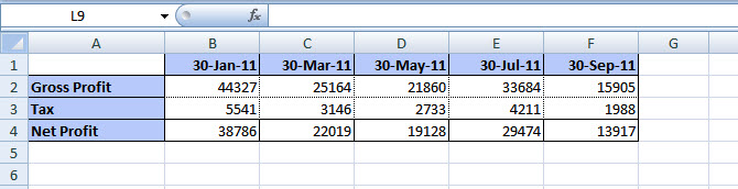
If you look at the image below it has few dates mentioned in column B to F and few figures for gross profit, tax & net profit associated with these dates.  Now what I am going to do is to sort these figures on the basis of dates in ascending order.

To do this what you'll have to do is follow a simple procedure and it will take very little time.  First of all select the data you want to sort and go to Home tab. There you'll find Sort & Filter option under Editing group.  Then you've to click on Custom Sort as shown in image below.

This will open a pop up box, at the top of it click on the Option button which will option Sort Options... box there look for Orientation and select Sort left to right.  By default it is Sort top to bottom.  This is shown in the image below.

Click OK and now you can see the option of sorting your data with rows.  Look at the sort by drop down option and you'll see Row1, Row2 etc now. Earlier it used to be Column1, Column2 and so on.

I've selected Row1, as my dates are in row 1 and I want to sort on their basis.  You can choose as per your requirement.  Oldest to Newest option under Order drop down will help us arrange the dates in required manner.  Click OK and here is what we intended to achieve.

Guys its easy and can be really helpful when you've to deal with large number of columns.  Hope you'll like my post, you can share your feedback or suggestion or any query via comments below. "HAPPY LEARNING"

MS Excel: Subtotal Function and Filter

The Subtotal function provide the subtotal of the numbers in a column.  It allows us to perform a calculation in the worksheet, and the same calculation can also be performed on the subsets of the data by applying filters. The magic of this function is that it ignores values in rows hidden by a filter.

The syntax for the Subtotal function is:

        Subtotal(function_num, ref1, ref2, ...)

function_num is the type of subtotal that you'd like to create. Image below explains 11 types which we can select:

ref1, ref2, ... are the ranges of cells that you want to subtotal.

Please go through the example with images below, it will help a lot in understanding Subtotal function.

Here I want to know the average monthly salary for each city. Normal AVERAGE function won't be helpful here because once we'll apply filter to it will still give us the average of all the records in the data. 

Now as per the requirement if I want to know the average monthly salary payable in Augusta region, the SUBTOTAL function will provide me the desired result while AVERAGE function will still give me the average of complete data.

I believe, I've not confused you and this post will be helpful to you while at work.  Let me know your feedback or suggestion.  I SHARE COZ I CARE! "Happy Learning"

Download SAMPLE FILE

VLOOKUP to fetch 2nd, 3rd or 4th Value

We all use VLOOKUP and must have observed a shortcoming that it only provides you with the first matching result. I mean if we have data where the lookup_value is coming twice or more times, VLOOKUP will give us the result for the first occurrence only. In the data below if your boss is interested in knowing the commission paid to "Mavericks Reality" for their second booking, how will you find that?

Solution will go like this:

You'll be a adding a helper column right next to broker's names and try to get a unique name. I am using COUNTIF function to do the trick for me like: =COUNTIF($B$2:B2,B2)&B2.

What this will do is, convert our lookup_values as 1Mavericks Reality, 2Mavericks Reality and so on (like in the image below). Now you have a unique lookup_value and you can simply use VLOOKUP("2Mavericks Reality",table_array,col_index) and you are done with your answer.

This is simple right?

You can download the sample file to get a better understanding of this tip. It tells you how you create formulae to get 2nd or 3rd occurrence. VLOOKUP FOR 2nd, 3rd OCCURRENCE.

Share this tip with everyone. "Happy Learning"

AND Function: Test Mathematical Conditions!

Moving ahead with our series of logical function, lets evaluate the AND function AND function provides result in TRUE or FALSE as output based on one of more condition. AND function evaluates at least one mathematical expression located in another cell in the spreadsheet.

The syntax it uses is as follow:

AND(logical1,logical2, ...)

Logical1, logical2, ...   are 1 to 255 conditions you want to test that can be either TRUE or FALSE.

Here is an example along-with image, it will help you understand the function in a better way.

I have few number in cell C1, C2 and C3 and I want to test certain mathematical conditions in cell D1 based on these numbers.

I have used the formula as follows

D1: =AND(C1>200,C2>200,C3>200)

If all three cells (C1,C2, and C3) has number greater than 200, the result in cell D1 will be TRUE. If any of these cells have value less than or equal to 200, the output for the AND function will be FALSE. "Happy Learning"

Explaining Array Formulas in Excel

There is special class of formulas available in Excel know as Array formulas or CSE b’coz they are entered by hitting three keys at a time Ctrl+Shift+Enter. There is no doubt this is one of the most powerful feature provided by Microsoft Excel, but this is one of least used feature as well. Array formulas empower you to calculate that you can’t perform with standard Excel function.  

The "Help" in Excel defines them as below:

"An array formula can perform multiple calculations and then return either a single result or multiple results. Array formulas act on two or more sets of values known as array arguments."

What motivated me to write on this post is also an interesting story. I have few very brilliant excel users as colleagues, one day one of them told me that he is not aware about the usage of array function. I tried to explain my bit, but he was not convinced with my elucidation.  That made me feels very strange! And decide to dedicate my next post to Array formulas.

I will not go into the details of this function and its application but will surely make you aware how it functions! So let visualize the data given below: 

and if I want you to know the sum of sales, provided more than 6 units are sold for Event product.

The function will go like this G13: = SUM((D2:D11="Event")*(E2:E11>6)*(G2:G11)) and hit Ctrl+Shift+Enter you will get the solution.

So array functions are helpful when we have more than one decisive factor for our result.

Important Tip! If your formula is not giving you the result you want and you believe you have done everything correctly, you can display the calculation in any part of your formula. To do so, just highlight the condition supplied and hit F9. 

It will give you result how Excel is seeing your condition in TRUE or FALSE.  It will give TRUE when the condition applies and FALSE where it fails.

This is a handy tip to remember for troubleshooting the parts of any formula that are giving you problems.

Before concluding this post I would like you to know the number one rule with array formula, use them only when needed and know when & where to use them. I am not trying to de-motivate you for using array formulas but too many arrays will slow down the functionality of your workbook.

And at last I would request to give your feedback for me and share posts with your contacts and social group.  Let’s continue enriching this mutual relation and help grow each other. “Happy Learning”

Two ways LOOKUP formula to extract values from left & right (INDEX & MATCH FUNCTIONS)

I am sure if you’re using Excel at work, then you must have used lookup function (LOOKUP, VLOOKUP & HLOOKUP). There is no doubt that these are most useful & beautiful functions provided in the excel package. But if you haven’t used these function yet, let me take the honor of telling you that a lookup function return a value from a given table by looking up another value in the same table.

Because of our habit of entering data in very common style, VLOOKUP is among the most used function of Excel. But there is a limitation that it cannot go left and with all the LOOKUP functions is that they only look in the left column and return a from a cell to the right. So what I mean by this is LOOKUP function in Excel are useful for one-way lookups, there is function (inbuilt) for two-way lookup.

Today after reading this post you will be able to conquer this limitation, I am sure of that! First I would like you to look at the data given below and visualize it. It a table representing sales figures for ten of my employees in USA. I have named this table as “SalesData”.

Now if you want to know whose region is Minnesota, no lookup function will be useful. This is because, LOOKUP functions only return values to the right and it doesn’t return values from the left side. One transitory solution can be cut the data from column C and insert it in column and use VLOOKUP, but such quick fix are not always possible. Especially when you are not supposed to manipulate the arrangement of data provided.

In this case we will take help of two functions available in Excel namely INDEX & MATCH.

INDEX(reference,row_num,column_num,area_num): This function returns the value of an element in a table or an array, selected by the row and column number indexes. It means this function will provide you result from your data when you supply the row number and column number of the desired result.  The answer will be intersection of supplied row & column number.

MATCH(lookup_value,lookup_array,match_type): This function returns the relative position of an item in an array that matches a specified value in a specified order. It means this function will provide you the number where your lookup value falls in the series.

Now let’s come back to our problem where we have to know the name of the sales person responsible Minnesota region.

The solution will go like this F13:  =INDEX(SalesData[Name],MATCH(D3,SalesData[Region],0)) this will provide the name as “JAMES”

Similarly if you want to know who over achieved his target by highest margin? Solution will be F14: =INDEX(SalesData[Name],MATCH(MAX(SalesData[Difference]),SalesData[Difference],0)) and the name will be “EMMA”.

Now before wrapping the post here I have some homework for you. Please try to find the following using function mentioned above.

• Who has the maximum & minimum target in my team and what were their respective regions? For minimum use MIN function.
• What is the name of person managing Kansas region and how long is he/she with the organization?
• Who has the lowest target among the team?
• Who is the newest member of the team?

Let me know you solutions, you can post them in the comment section!

I hope you like this post and will share this with your friends and colleagues to help us grow the community of excel learners, there are various options you can use to share with people at the end of the post.

Now you also follow me on Twitter, just click on the vertically aligned Twitter radio button to the left of your computer screen to follow!

You can post your feedback as a comment below and I will take a note of it for future. “Happy Learning”

Please download the file from here!

Create a Table in Excel 2007

With the launch of Office 2007, Microsoft has introduced a rich concept to Excel know as "Table". Table in Excel 2007 help you to manage and analyze your data. This feature has less functionality in terms of calculation but it is very useful in storing lots of information consistently. Formatting, sorting and filtering are very easy with Table. Typically, an Excel table has only column headings and no row headings.
 

I would recommend you to organize your data before creating a Table. Few points which you keep in mind are as follows:

• Your data should have a proper and unique heading in column
• There should be no blank row or column in your data
• Your data should be separated with any other information by at least one row and one column

How to create a Table?

Creating a table is very easy in excel.

1. Select the cells that contain data

2. On the Ribbon, click the Insert tab and in the Tables group, click the Table command

3.Click OK and you are done with a default style table

Special functionality of a Table 

• Autofilter and Sort: When you create a Table it provides you with integrated Autofilter and Sort functionality to your data. You don't have to add this feature manually, only this that is required to make it more helpful is your data should have headings in each column.
• Header names while scrolling: If your data is large and it doesn't fit your screen while scrolling new Excel has feature that temporarily replace column letters with the table's column names.
• Automatic expansion of data: When you add new data in row or column of your table, Excel expands the range of your table and takes it as part of your table.
• Automatic formatting: When you add or delete any row into the table it automatically formats the change. You don't have to make edits to the changed data Excel Table will do it for you! 

I hope you find my posts helpful and easy to learn at the same time. Please do share the tips with your friends, colleagues and if you have any feedback for me I will look forward to it. 

"Happy Learning"

Excel Function: IF ( logical_test, value_if_true, value_if_false )

Now in coming two weeks I have decided to discuss functions available in the stable of Microsoft Excel.  I have taken Logical function to start with, as I found them most useful will working data (this is my personal view :) though). To start with I am gonna explain IF function with an example.

The IF function is one of Excel's logical functions and it tests to see if a certain condition in a spreadsheet is true or false.

The syntax for the IF function is:

=IF (logical_test, value_if_true, value_if_false)

logical_test    - a value or expression that is tested to see if it is true or false.
value_if_true  - the value that is displayed if logical_test is true.
value_if_false - the value that is displayed if logical_test is false.

Some of the conditional operator you need to know:
<   - Less Than
>= - Greater than Or Equal To
<= - Less than Or Equal To
<> - Not Equal To

The following two images will tell you how we can use IF function. In cell A1 have value 15 and I want to populate test "Good" or "Bad" based on this value. For example if value is greater than 10 then it is "Good" else "Bad".

 

Formula which I have entered in cell A2: =IF(A1>10,"Good","Bad")

Similarly you can see cell B2 is giving me "Bad" because A2 is less than 10.

You can use this many ways and under numerous conditions. Few days back one of my teacher friend came to me and we were discussing how we can use Excel to help him in work. He gave me a situation where based on a number he wants to assign grades to his student. The parameters to grades were as follows:

A If the student scores 85 or above
B If the student scores 65 to 84
C If the student scores 50 to 64
D If the student scores 33 to 49
FAIL If the student scores below 33

An example of this data looks like this:
To solve his problem I used IF Function. I created a similar table below his data and wrote a formula as B12: =IF(B2>=85, "A", IF(B2>=65, "B", IF(B2>=50, "C", IF(B2 >=33, "D", "Fail" ) ) ) )

I draged the formaula cross the data sheet and got my result.

I hope this is clear to everyone. I know many of you are already using this function.  Kindly let us know how do you use this function in your daily life.  You can post your experiences and example in the comment box, it will help us in learning new things.  "Happy Learning"

Pass this to your friends and colleagues this may also help them! 

To download the example file click here

Create charts directly in a range

This post will be talking about how to create non-graphic chart without using the default chart templates in Excel.  This method use combination of functions to display bars in the call corresponding to the data.

In the screen-shot above, I have data containing targeted (column B) and actual (column C) number of calls made by agents  in an assessment period. Column D represents, the variance of their performance (in %). 

Functions I have used to create this are IF, REPT, FLOOR & ABS.

To re-create this chart in Excel, please have your data handy or enter the data shown in columns A through D, and then write the following formulas:

E2: =IF(D2<0,REPT("g ",FLOOR(ABS(D2*100),1)),"")

F2: =A2

G2: =IF(D2>0,REPT("g ",FLOOR(ABS(D2*100),1)),"")

I have used webdings font to cells E2 an G2, but you can play here with your imagination (can insert as well). Copy the formulas and paste till the end. Right-align the text in column E, and Left-align in column G.

To make the chart presentable specially when your data contain large variances, you will have to adjust the scaling.  That can be achieved by dividing your result of FLOOR function by any number that suits your presentation.

For example in your function;

E2: =IF(D2<0,REPT("g ",FLOOR(ABS(D2*100),1)),""),  "FLOOR(ABS(D2*100),1)" is giving you a high value such as 50 to make it presentable you can adjust the function by diving the result by 5.  So the new function will be IF(D2<0,REPT("g ",FLOOR(ABS(D2*100),1)/5),"") you can change this divisor to any number you want.

I hope you learnt something interesting with the post. "Happy Learning"

Excel Function: MROUND (Rounding value to a multiple)

Readers if you want to round a value to some multiple of a whole number, you need to know MROUND function.  It works wonders when it comes to round a value with respect to a given multiple. The MROUND function can be used to round a number up or down to a specified multiple.

The syntax for the MROUND function is as follows:
=MROUND (Number, Multiple)

 
Number: the number which you want to round up or down

 
Multiple: the number provided will be rounded up or down in multiple of this figure.  Number will be rounded up if the last digit is more or equal to 5. If it is less than 5, it will be rounded down.

Another important thing you should know is that both number and multiple should have same sign. Either positive or both bearing negative sign else the function will give #NUM! Error.

You can find this function under Formulas tab of the ribbon menu. There you choose Math & Trig and click on MROUND in the list.

In Excel 2007 (and later) this function has been removed from the Analysis ToolPak add-in and is available as standard. For people using Excel 2003 or earlier, this function is only available when you have the Analysis ToolPak add-in loaded.

In the below screenshot I have tried to incorporate all possible examples:

I hope you all will be benefitted with MROUND function.  Happy Learning!

Excel Function: DATEDIF (Explaining DATEDIF function with Images.)

The DATEDIF function calculates the difference between two dates in number of ways, such as years, months, or days between the entered dates. You will not find this function in Formulas tab but it there in excel. To use, you’ll have to type it manually in any cell. The syntax for DATEDIF is as follows:

=DATEDIF(DateA, DateB, Interval)

Where:
DateA is the first date,
DateB is the second date,
Interval is the interval type to return.

The Interval value should be one of the following:

• "d" means Days (Number of days between the dates.)
• "m" means Months (Complete calendar months between the dates.)
• "y" means Years (Complete calendar years between the dates.)
• "ym" means Months Excluding Years (Complete calendar months between the dates as if they were of the same year.)
• "yd" means Days Excluding Years (Complete calendar days between the dates as if they were of the same year.)
• "md" means Days Excluding Years And Months (Complete calendar days between the dates as if they were of the same month and same year.)

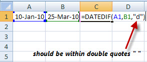
The Interval should be within “_”double quotes when Interval string is being entered directly within the formula:

=DATEDIF(DateA,DateB,"d")

When you have interval in another cell referenced in the formula, that cell should not have double quotes around the Interval string. For ex,

=DATEDIF(DateA,DateB,C1)

cell C1 should contain d not "d".
 

Best Usage: Calculating Age
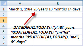
When you have to calculate your age as of today DATEDIF is of great use. It not simplifies the process and provide presentable figure. For example, formula below will give result in cell B2 the age of a person as of the current date, where cell A1 contains person's date of birth.

B1: =DATEDIF(A1,TODAY(),"y")&" years "&DATEDIF(A1,TODAY(),"ym")&" months "&DATEDIF(A1,TODAY(),"md")&" days"

We sometime need to know exact age as on any specific date, commonly while applying for government jobs which has a upper limit for age as a eligibility criteria. DATEDIF function can also be used to ease out the problem as follows:

C2: =DATEDIF(A2,B2,"y")&" years "&DATEDIF(A2,B2,"ym")&" months "&DATEDIF(A2,B2,"md")&" days"

That’s it for now, will post more soon. Comments and questions are welcome. Till then, “Learn & Grow Together with EXCEL”

Fill in Blank Cell from Cell Above

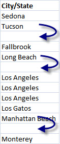
Objective is to fill all the blank cells in a column with the Data from the above cell.  Below images can explain it in a better way:

To solve this problem there can be many ways, hardest and very time consuming being copying and pasting data manually specially when you're dealing with large data.  We can write 'n' number of formula's to solve this, but I am going to tell a very simple and quick method of doing it.

Here we go, 

• First select all the columns containing your data
• Press Ctrl+G or F5 this will open Go To dialogue box

• Press Special... and a new dialogue box will pop out

 

• This will select all the blank cell in your data and Type "=" and then hit up arrow for example A4: =A3

 

• Press Cltr+Enter to input that formula into all currently selected blank cells.

  And we are done in a flash.

This appears simple to me, Let me know what do you think.