Excel Function: MROUND (Rounding value to a multiple)

Readers if you want to round a value to some multiple of a whole number, you need to know MROUND function.  It works wonders when it comes to round a value with respect to a given multiple. The MROUND function can be used to round a number up or down to a specified multiple.

The syntax for the MROUND function is as follows:
=MROUND (Number, Multiple)

 
Number: the number which you want to round up or down

 
Multiple: the number provided will be rounded up or down in multiple of this figure.  Number will be rounded up if the last digit is more or equal to 5. If it is less than 5, it will be rounded down.

Another important thing you should know is that both number and multiple should have same sign. Either positive or both bearing negative sign else the function will give #NUM! Error.

You can find this function under Formulas tab of the ribbon menu. There you choose Math & Trig and click on MROUND in the list.

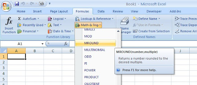
In Excel 2007 (and later) this function has been removed from the Analysis ToolPak add-in and is available as standard. For people using Excel 2003 or earlier, this function is only available when you have the Analysis ToolPak add-in loaded.

In the below screenshot I have tried to incorporate all possible examples:

I hope you all will be benefitted with MROUND function.  Happy Learning!

Excel Function: DATEDIF (Explaining DATEDIF function with Images.)

The DATEDIF function calculates the difference between two dates in number of ways, such as years, months, or days between the entered dates. You will not find this function in Formulas tab but it there in excel. To use, you’ll have to type it manually in any cell. The syntax for DATEDIF is as follows:

=DATEDIF(DateA, DateB, Interval)

Where:
DateA is the first date,
DateB is the second date,
Interval is the interval type to return.

The Interval value should be one of the following:

• "d" means Days (Number of days between the dates.)
• "m" means Months (Complete calendar months between the dates.)
• "y" means Years (Complete calendar years between the dates.)
• "ym" means Months Excluding Years (Complete calendar months between the dates as if they were of the same year.)
• "yd" means Days Excluding Years (Complete calendar days between the dates as if they were of the same year.)
• "md" means Days Excluding Years And Months (Complete calendar days between the dates as if they were of the same month and same year.)

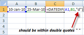
The Interval should be within “_”double quotes when Interval string is being entered directly within the formula:

=DATEDIF(DateA,DateB,"d")

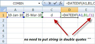
When you have interval in another cell referenced in the formula, that cell should not have double quotes around the Interval string. For ex,

=DATEDIF(DateA,DateB,C1)

cell C1 should contain d not "d".
 

Best Usage: Calculating Age
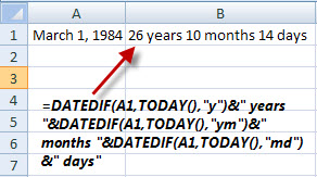
When you have to calculate your age as of today DATEDIF is of great use. It not simplifies the process and provide presentable figure. For example, formula below will give result in cell B2 the age of a person as of the current date, where cell A1 contains person's date of birth.

B1: =DATEDIF(A1,TODAY(),"y")&" years "&DATEDIF(A1,TODAY(),"ym")&" months "&DATEDIF(A1,TODAY(),"md")&" days"

We sometime need to know exact age as on any specific date, commonly while applying for government jobs which has a upper limit for age as a eligibility criteria. DATEDIF function can also be used to ease out the problem as follows:

C2: =DATEDIF(A2,B2,"y")&" years "&DATEDIF(A2,B2,"ym")&" months "&DATEDIF(A2,B2,"md")&" days"

That’s it for now, will post more soon. Comments and questions are welcome. Till then, “Learn & Grow Together with EXCEL”

Fill in Blank Cell from Cell Above

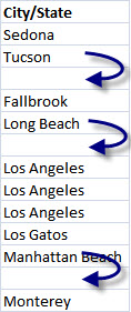
Objective is to fill all the blank cells in a column with the Data from the above cell.  Below images can explain it in a better way:

To solve this problem there can be many ways, hardest and very time consuming being copying and pasting data manually specially when you're dealing with large data.  We can write 'n' number of formula's to solve this, but I am going to tell a very simple and quick method of doing it.

Here we go, 

• First select all the columns containing your data
• Press Ctrl+G or F5 this will open Go To dialogue box

• Press Special... and a new dialogue box will pop out

 

• This will select all the blank cell in your data and Type "=" and then hit up arrow for example A4: =A3

 

• Press Cltr+Enter to input that formula into all currently selected blank cells.

  And we are done in a flash.

This appears simple to me, Let me know what do you think.